CMR usage on example data set

Volker J Schmid

2023-07-18

Simulate cmr data

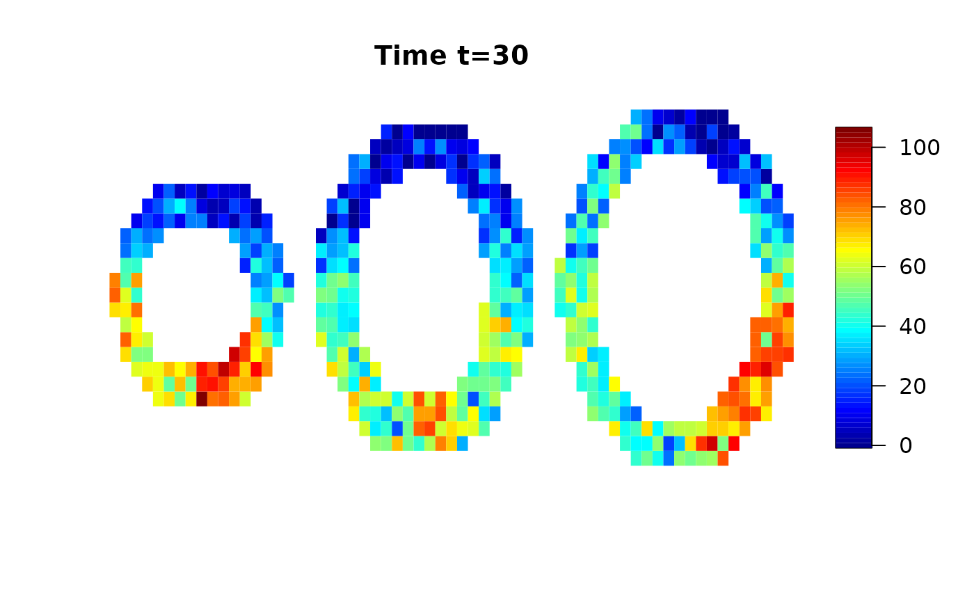
We use a simulated data set provided by the cmR package and add random white noise.

data(cmrsim)
for (i in 1:dim(cmrdata_sim)[1])
for (j in 1:dim(cmrdata_sim)[2])
for (k in 1:3)
if (!is.na(cmrdata_sim[i,j,k,1]))
cmrdata_sim[i,j,k,]=cmrdata_sim[i,j,k,]+rnorm(30,0,sqrt(30))

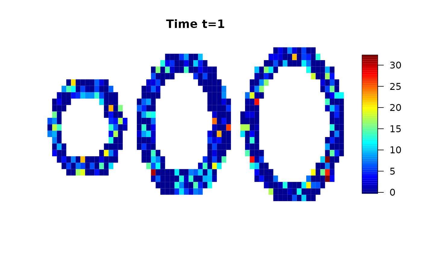
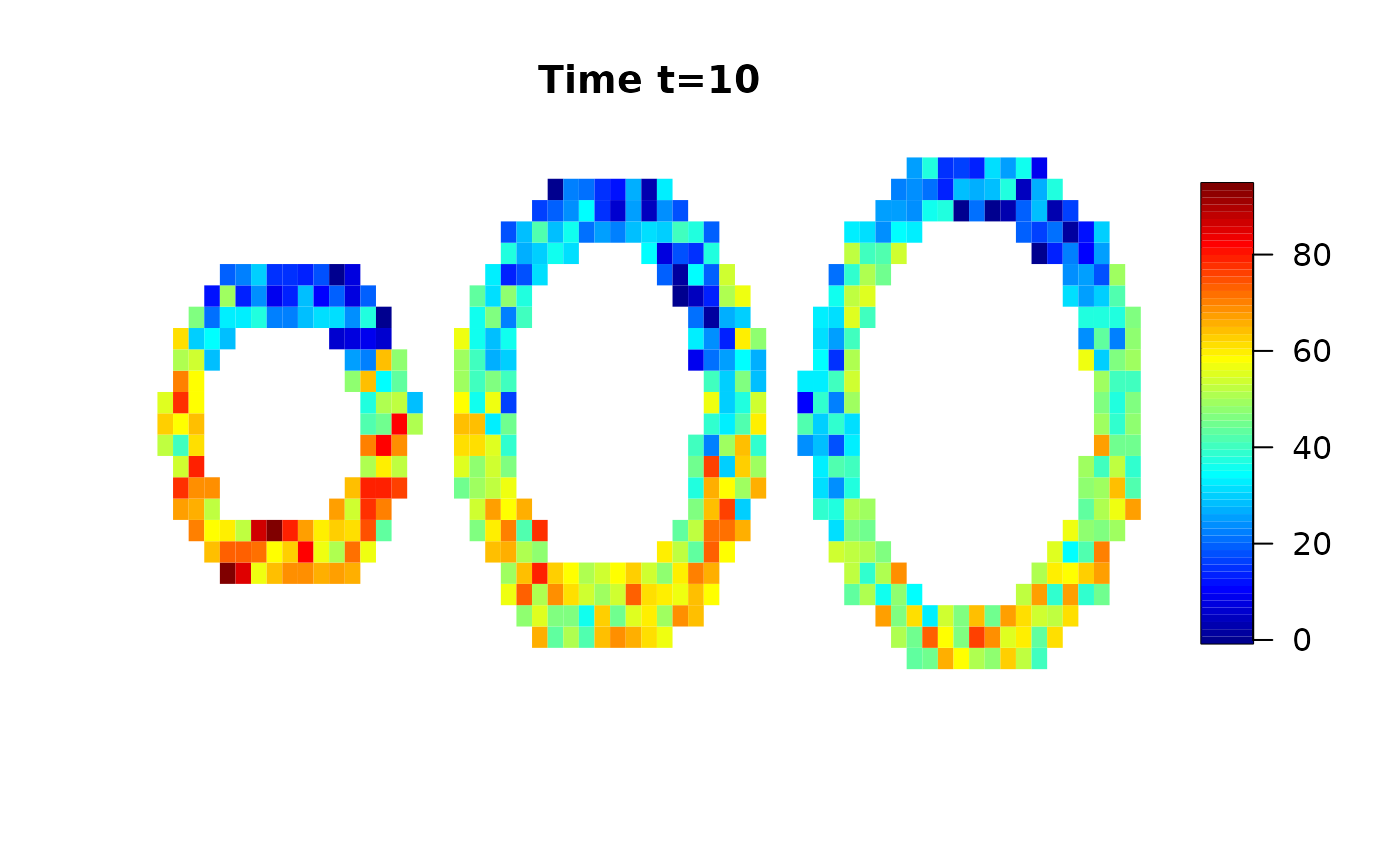
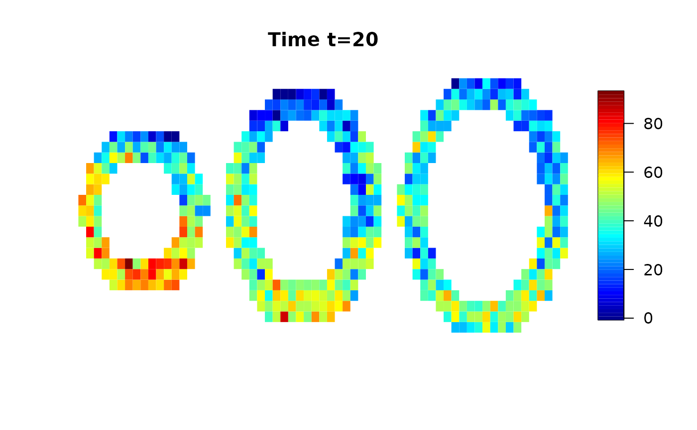
Let’s have a look on the data:

imageMBF(cmrdata_sim[,,,1])
title(main="Time t=1")

imageMBF(cmrdata_sim[,,,10])
title(main="Time t=10")

imageMBF(cmrdata_sim[,,,20])
title(main="Time t=20")

imageMBF(cmrdata_sim[,,,30])
title(main="Time t=30")

Analysis

The function cmr() does the analysis and provides two methods: “local”, which is a voxel wise fitting of the time series and “spatial”, which uses the spatial prior used in Schmid (2011): Voxel-Based Adaptive Spatio-Temporal Modelling of Perfusion Cardiovascular MRI. IEEE TMI 30(7) p. 1305 - 1313.

Here we start with the local analysis. The local analysis can be easily parallelised, each computer core can compute one voxel. Note: parallel computing cannot be used on Windows due to restrictions in the parallel package.

local=cmr(cmrdata_sim,input_sim,method="local",cores=2)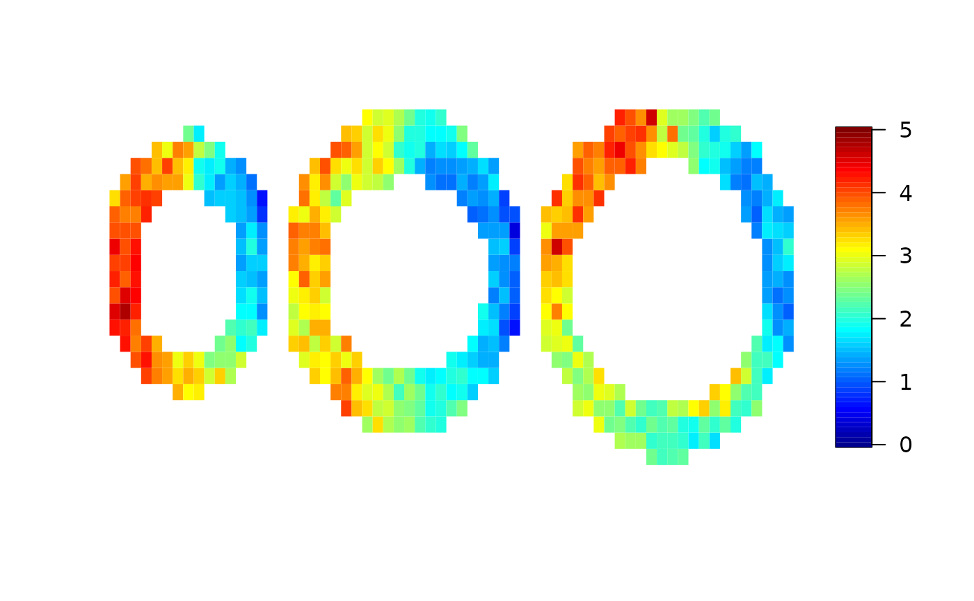

imageMBF(local$mbf,zlim=c(0,5))

The model uses a Bayesian framework and credible intervals are also produced. We can have a look at the length of the credible intervals voxelwise:

imageMBF(local$ci,zlim=c(0,.8))

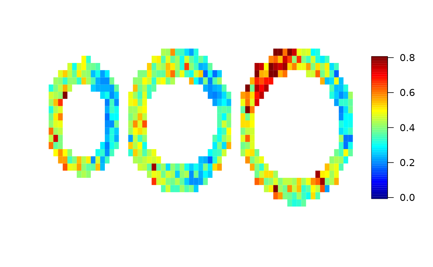
Now let’s have a look at the spatial analysis. Here, parallelisation is not as easy as above, but is also possible to some extent.

spatial=cmr(cmrdata_sim,input_sim,method="spatial",cores=2)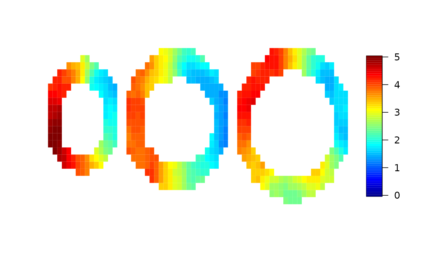

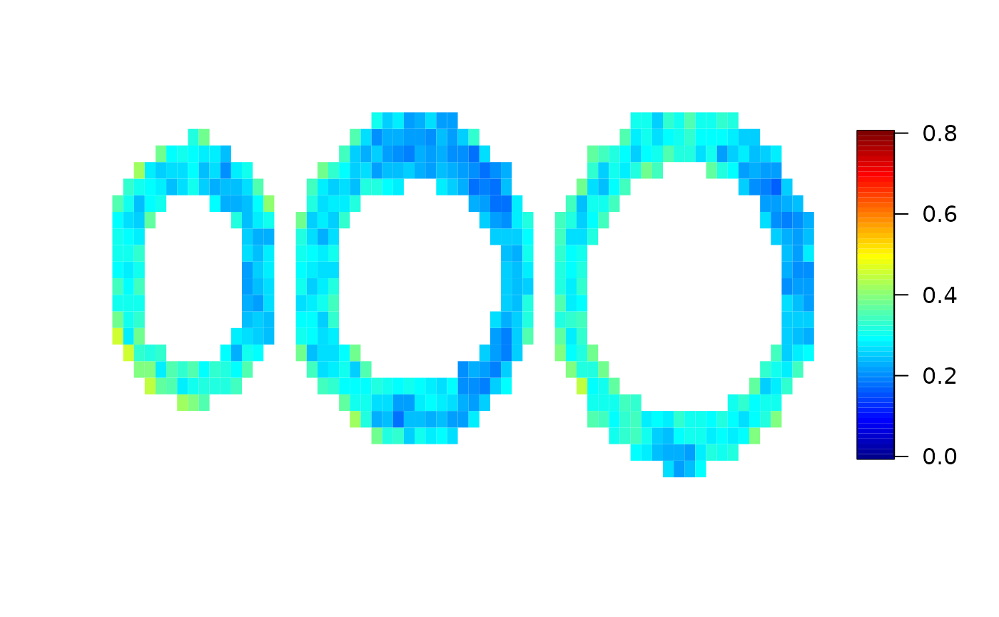
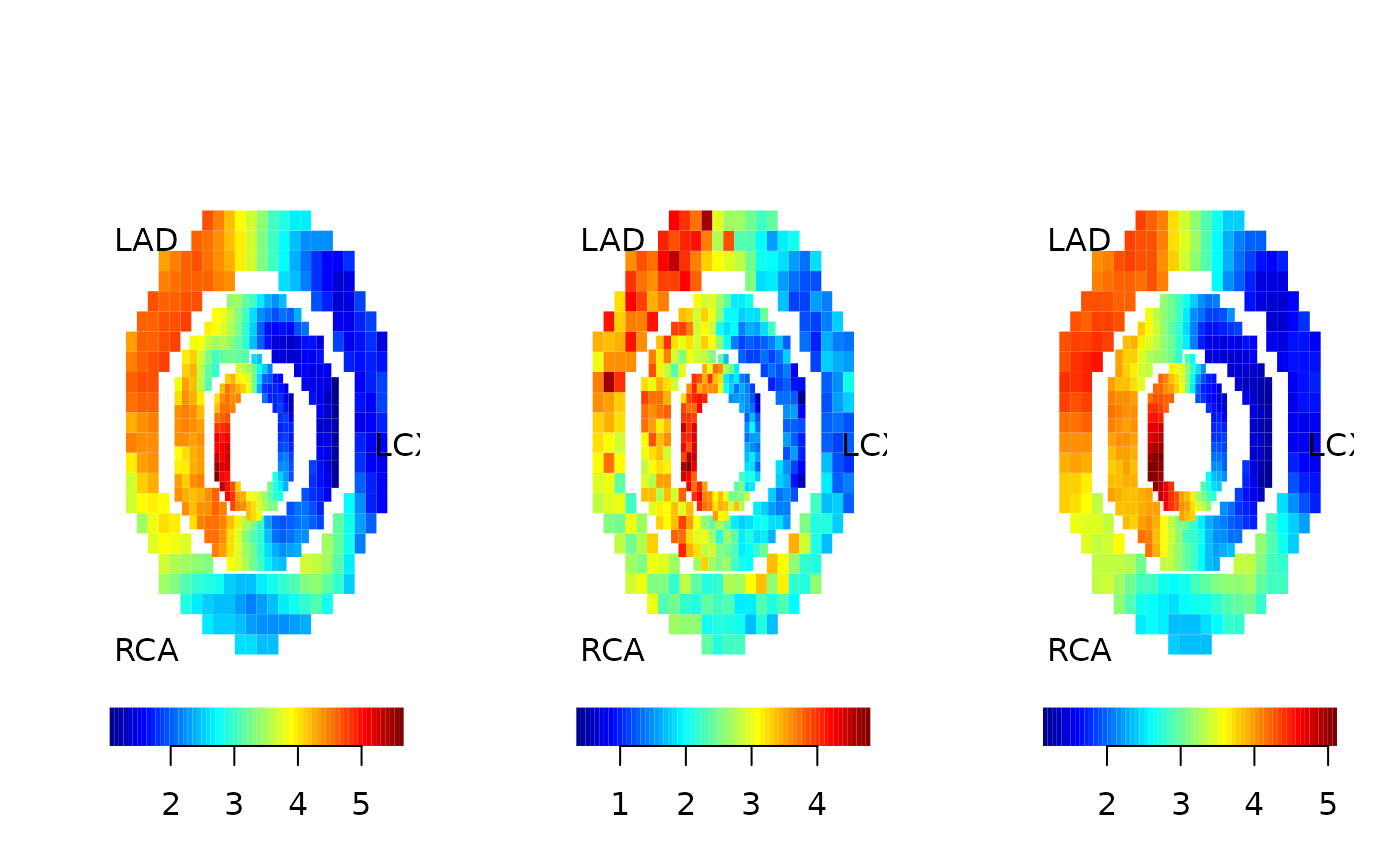
imageMBF(spatial$mbf,zlim=c(0,5))

imageMBF(spatial$ci,zlim=c(0,.8))

Finally, we compare the true maximum response used for the simulation and the results from the local analysis and the spatial analysis. Here, we use the “pseudo bullseye” representation.

par(mfrow=c(1,3))
pseudobullseye(maxresp_sim)#; title(main="true")
pseudobullseye(local$mbf)#; title(main="local")
pseudobullseye(spatial$mbf)#; title(main="spatial")